Creating databases and tables for Athena
Posted: | Tags: aws til athenaBen Welsh and Katlyn Alo have created a course that walks through running your first Athena query, complete with sample data. I’ve written about Athena a few times on this blog and the course works as a great primer. This post will act as an addendum to the guide, specifically step 4, where you create an Athena database and table.
A database, in Athena, holds one or more tables, and the table points to the data and what schema it’s in. The creation of these resources in the guide follows a pattern I’ve seen a lot where the database and table are created using SQL through Athena. It’s simple, and does the job, but I’d like to document how to create a table and database using AWS Glue, an extract-transform-load data service, and highlight some comparisons between the two methods.
Create databases and tables through Athena
To start, creating the database and table through the Athena editor using SQL is quite straightforward and I won’t go over this in detail as it’s already well covered by the guide in step 4.
Creating a database is done through the CREATE DATABASE statement, and replacing DATABASE_NAME with your desired name.
CREATE DATABASE DATABASE_NAME
Creating a table uses the CREATE EXTERNAL TABLE statement. Where this can get complicated is when defining your data’s schema, especially if you’re using a complex dataset. For the purposes of the course the dataset was already well documented and easy enough to define while referencing the available data types in Athena.
Once created you can use the table to query your data using SQL.
Create databases and tables through AWS Glue
An alternative way to create the database and table is through AWS Glue. Within Glue, a crawler is used to crawl a data store and create tables on your behalf within a database. Using a Glue crawler has the advantage of automatically defining the data schema, and partitioning the data to make queries run more efficiently, in other words, faster and cheaper. While both, the schema and partitions, can be defined manually it can be difficult. Let’s look at creating a crawler for the dataset used in the guide.
Create a table using a Glue Crawler
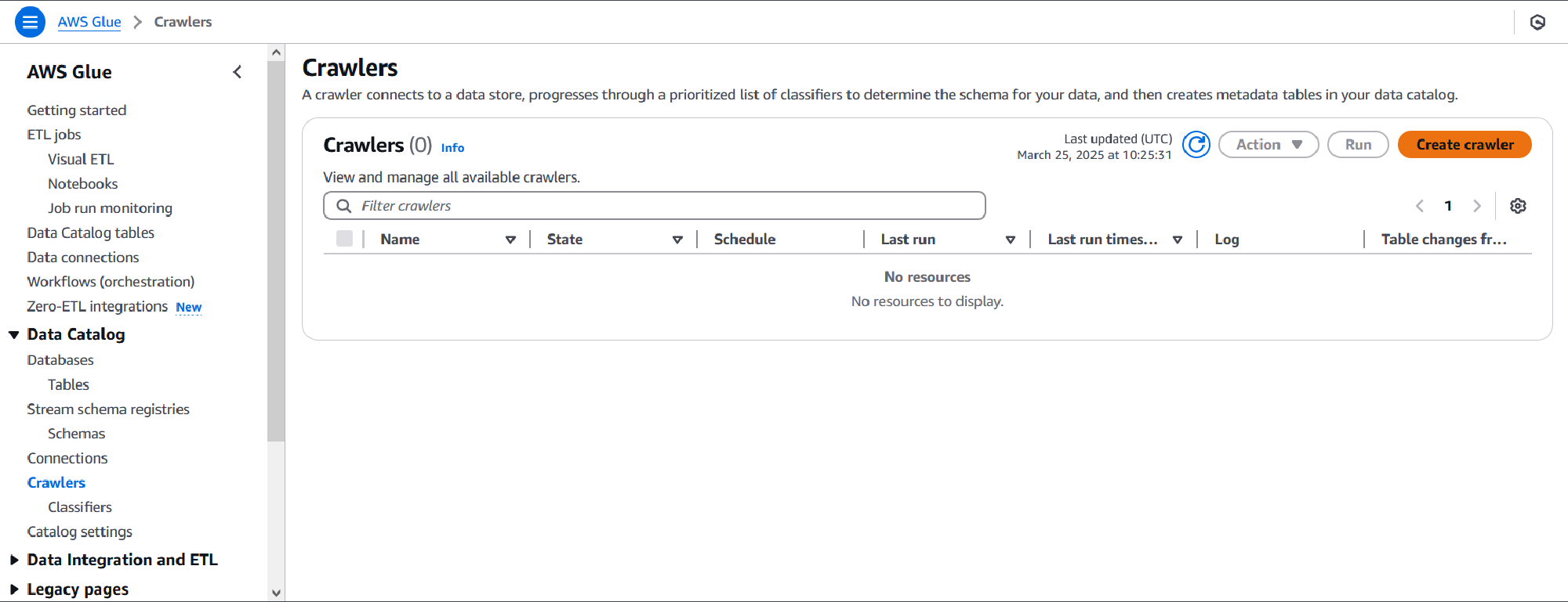
Go to the AWS Glue console, by searching for Glue at the top. From the left navigation menu, of the Glue console, select Crawlers under the Data Catalog dropdown and then the orange Create crawler button.
On the crawler properties page, set a name and optionally a description.

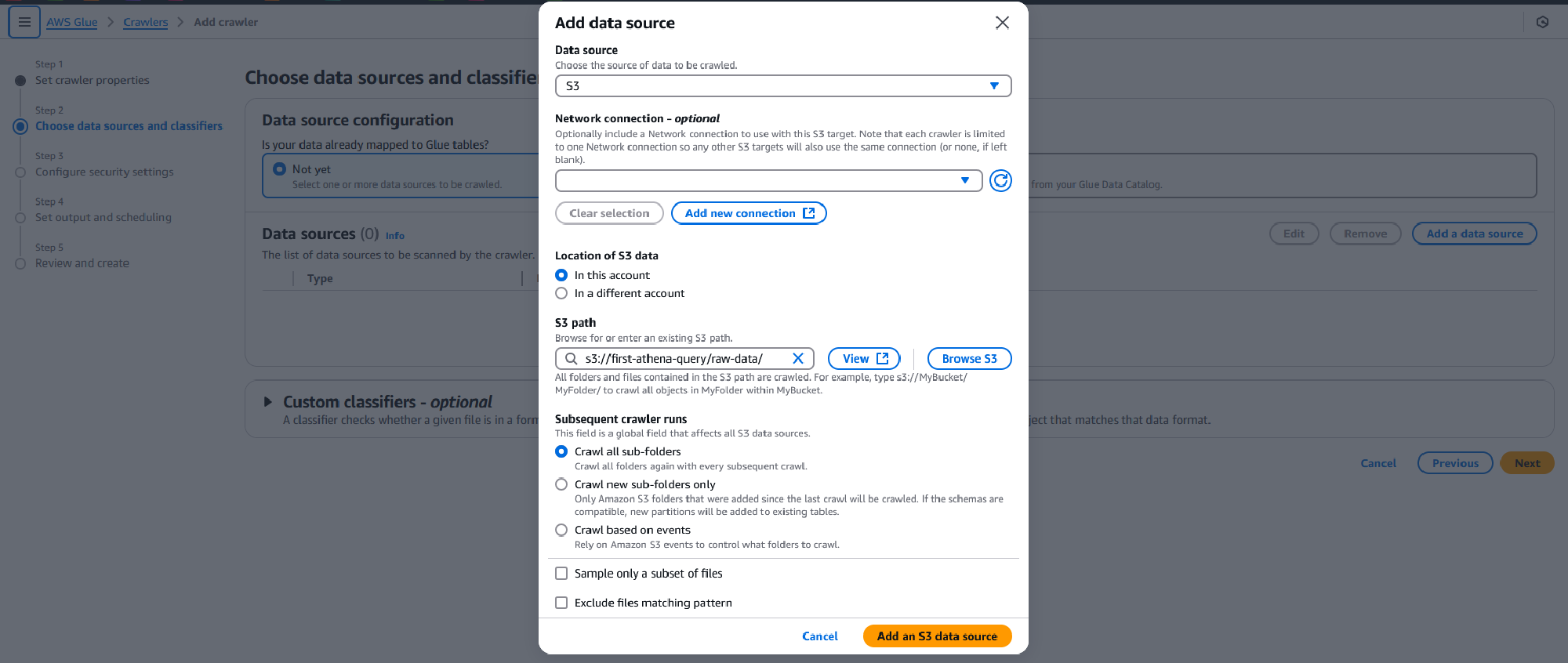
On the next page, click the Add a data source button, and Browse S3 for the S3 bucket and folder used to store the data set. All other options on this page can be left as-is. For data that is incrementally updated in new folders, you can choose to set the Subsequent crawler runs to Crawl new sub-folders only reducing crawl time (and costs). Click Add S3 data source and Next once you are finished.
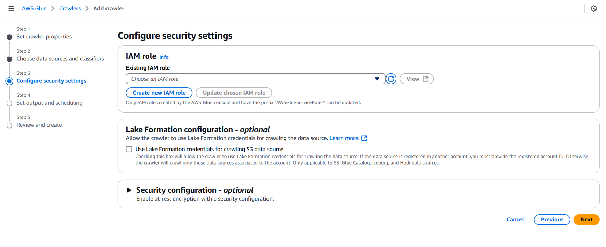
On the security settings page opt to Create new IAM role by clicking the blue button and enter a name for the role. This will create a role with permissions for the Glue crawler to parse through your dataset in S3. Click Create and Next once you are finished.
On the next page, you can set your output configuration and crawler schedule. The output includes the Target database, this could be one you created previously through Athena, in which case you can choose it from the dropdown, or you may opt to create one through Glue.
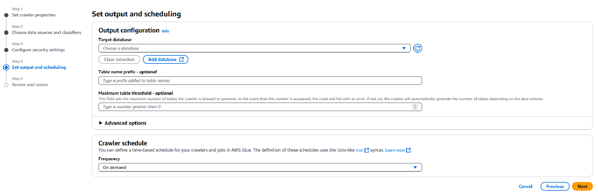
If it’s the latter, click the Add database button, this opens a new tab where you can enter the database name and optionally a description, once done click Create database. Return back to the Crawlers tab, click the blue refresh button and select the newly created database from the dropdown.
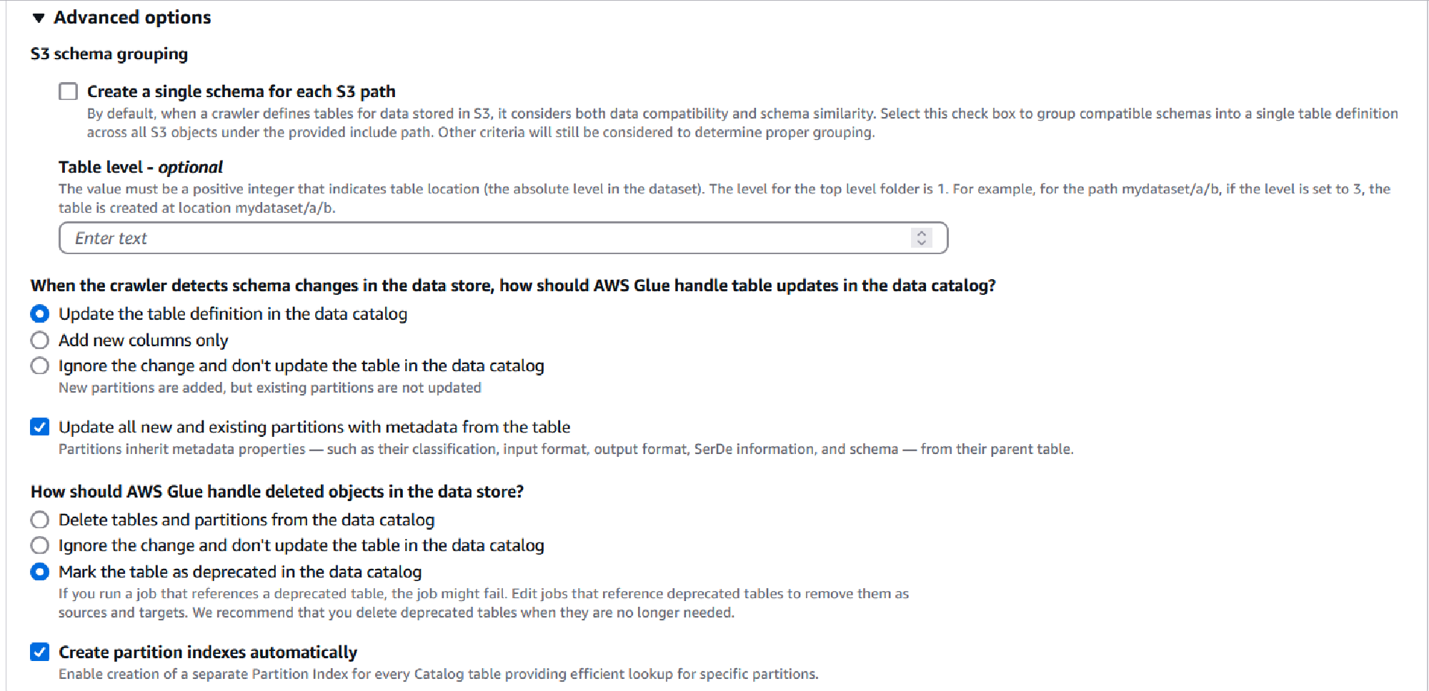
Under Table name prefix - optional, you may enter a prefix for the table Glue will create. By default it chooses the name of the root folder in your S3 bucket, I will prefix that with “loans_” to make it more human-readable later.
Under the Advanced options dropdown there are many options to configure your crawler, two I’d like to point out are to update metadata for existing partitions and create partition indexes automatically. The first may be relevant if your data schema changes within your dataset or needs to be updated between crawls to include more columns or changes in data type, the second helps with efficient queries.
Lastly, I will leave the Crawler schedule to On demand but you may wish to change this later based on how frequently you update your dataset partitions. Once ready click Next.
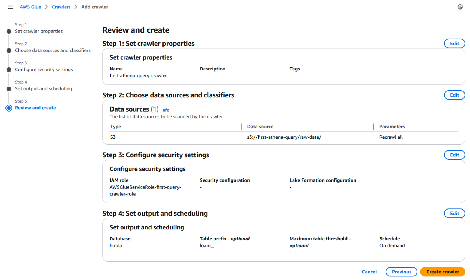
On the final page, review all the options selected and click Create crawler.
You will now be redirected to your crawler page, where you will be able to browse through all the parameters you set. Click on Run crawler to begin your first run. This should take approximately 1 minute if you are using the sample dataset from the guide. The status under Crawler runs will change to Completed once done.
You have now created a table from AWS Glue! It may seem like a lot of steps, but it’s mostly clicking through dialogue boxes and becomes simpler as you get familiar with the interface.
Table schema
The Glue Crawler can parse and understand data formats through classifiers. There are many built-in classifiers that support popular formats like CSV, JSON, XML and even some logs files, you have the option to create and use your own classifiers for unsupported formats. By crawling through the dataset Glue has created a table, along with the schema, the data types selected automatically almost match what was manually created in the guide. An example where they differ is with country_code, Glue picked bigint whereas the guide rightfully picked string, as we do not intend to do any mathematical calculations on the numbers themselves string works fine. Data types can be adjusted through the Glue console by selecting your table under the Data Catalog dropdown from the left navigation pane end editing the schema.
For reference, the table below compares what was picked for each column’s data type automatically by Glue and what was defined through the SQL query in the guide.
| Column | Data type (Glue) | Data type (manual) |
|---|---|---|
| activity_year | bigint | int |
| lei | string | string |
| state_code | string | string |
| county_code | bigint | string |
| census_tract | bigint | string |
| derived_loan_product_type | string | string |
| derived_dwelling_category | string | string |
| derived_ethnicity | string | string |
| derived_race | string | string |
| derived_sex | string | string |
| action_taken | bigint | int |
| purchaser_type | bigint | int |
| preapproval | bigint | int |
| loan_type | bigint | int |
| lien_status | bigint | int |
| reverse_mortgage | bigint | int |
| open_end_line_of_credit | bigint | int |
| business_or_commercial_purpose | bigint | int |
| debt_to_income_ratio | string | string |
| applicant_credit_score_type | bigint | string |
| partition_0 | string | N/A |
In most scenarios, this is, by far, the biggest benefit of using a crawler instead of manually defining the schema in the Athena editor.
Partitions
Partitions in a table segments the data to be efficiently queried, this can reduce the amount of data scanned per query and subsequently the time taken to return a result. A Glue crawler will automatically determine when to create partitions based on the folder structure, this can be adjusted by specifying the partitioning level within the crawler options.
In our example dataset, by default, the table will be partitioned by year given the folders under the top-level folder created by the dataset script from the guide represent the loan years. The partition will be unable to recognize the folder names are years, and so will be called “parition_0”, you can see this in the last row of the table above.
One thing to keep in mind is when a new year is added you will need to re-run the crawler to partition the newly added data, otherwise it will not be available to query. This is one downside compared to simply defining the schema using SQL, although you may also wish to use no partition with the crawler. Should you wish to automate running the crawler, you can set it to run on a schedule, manually trigger it or configure it to respond to S3 upload events.
To test the claims of efficiency, I crafted a sample query, based on the query used in the guide, that sum of each loan type in 2018 across all counties. For the manually created table, this query looks like the following:
SELECT
    SUM(CASE WHEN loan_purpose = 1 THEN 1 ELSE 0 END) as "Home purchase",
    SUM(CASE WHEN loan_purpose = 2 THEN 1 ELSE 0 END) as "Home improvement",
    SUM(CASE WHEN loan_purpose = 31 THEN 1 ELSE 0 END) as "Refinancing",
    SUM(CASE WHEN loan_purpose = 32 THEN 1 ELSE 0 END) as "Cash out refinancing",
    SUM(CASE WHEN loan_purpose = 4 THEN 1 ELSE 0 END) as "Other purpose",
    SUM(CASE WHEN loan_purpose = 5 THEN 1 ELSE 0 END) as "N/A",
    COUNT(*) as "Total"
FROM "hmda"."loans"
WHERE activity_year = 2018
For the Glue created database and table, I’ve modified the query to use “partition_0” instead of “activity_year”, also note that the year here is a string instead of an integer as was manually defined.
SELECT
    SUM(CASE WHEN loan_purpose = 1 THEN 1 ELSE 0 END) as "Home purchase",
    SUM(CASE WHEN loan_purpose = 2 THEN 1 ELSE 0 END) as "Home improvement",
    SUM(CASE WHEN loan_purpose = 31 THEN 1 ELSE 0 END) as "Refinancing",
    SUM(CASE WHEN loan_purpose = 32 THEN 1 ELSE 0 END) as "Cash out refinancing",
    SUM(CASE WHEN loan_purpose = 4 THEN 1 ELSE 0 END) as "Other purpose",
    SUM(CASE WHEN loan_purpose = 5 THEN 1 ELSE 0 END) as "N/A",
    COUNT(*) as "Total"
FROM "hmda_glue"."loans_raw_data"
WHERE partition_0 = '2018'
Running each query three times without partitioning resulted in an average run time of 5.8 seconds and with partitioning the the average was 1.7 seconds. Looking at the data scanned, without partitioning as expected all 15.52GB of data was scanned each time whereas with partitioning only 2.42GB of the 2018 dataset was scanned.
And we have it, an outline to set up a crawler, and their subsequent results. This small test cost $0.03 with Glue in time spent crawling, and $0.58 with Athena to scan the data for the queries I ran (I ran a few more than the two I shared). I’d suggest reading the respective pricing pages to get more details. There’s a lot more to be said, but we’ve covered everything I’d intended to and now I have somewhere to link to when I talk about using Glue and Athena together.